Electromagnetic Flow Meter
- Home
- Electromagnetic Flow Meter
Electromagnetic Flow Meter

Key Features
Measurement Principle
• Based on Faraday’s Law of Electromagnetic Induction
• Generates voltage proportional to fluid velocity
• Ensures highly reliable and linear measurement
• Generates voltage proportional to fluid velocity
• Ensures highly reliable and linear measurement
Accuracy & Performance
• Accuracy: ±0.2% to ±0.5% of reading
• Repeatability: ±0.1%
• Stable measurement even under fluctuating flow conditions
• Not affected by density, viscosity, temperature, or pressure
• Repeatability: ±0.1%
• Stable measurement even under fluctuating flow conditions
• Not affected by density, viscosity, temperature, or pressure
Flow Capability
• Bidirectional flow measurement
• Wide velocity range: 0.1 to 10 m/s (up to 15 m/s max)
• Suitable for low to high flow rates
• Wide velocity range: 0.1 to 10 m/s (up to 15 m/s max)
• Suitable for low to high flow rates
Fluid Compatibility
• Suitable for conductive liquids (≥ 5 μS/cm)
• Ideal for water & wastewater, slurries, sewage
• Suitable for chemicals, acids, and food & beverage liquids
• Performs well with dirty, corrosive, and abrasive fluids
• Ideal for water & wastewater, slurries, sewage
• Suitable for chemicals, acids, and food & beverage liquids
• Performs well with dirty, corrosive, and abrasive fluids
Construction & Materials
• Full bore design (no obstruction, no pressure loss)
• Liner materials: PTFE, PFA, Rubber / EPDM
• Electrode materials: SS316, Hastelloy C, Titanium, Tantalum
• Liner materials: PTFE, PFA, Rubber / EPDM
• Electrode materials: SS316, Hastelloy C, Titanium, Tantalum
Size & Installation
• Available sizes: DN10 to DN2000 and above
• Connections: Flanged, Wafer type, Threaded
• Requires full pipe condition for accurate measurement
• Reduced straight pipe requirement compared to other meters
• Connections: Flanged, Wafer type, Threaded
• Requires full pipe condition for accurate measurement
• Reduced straight pipe requirement compared to other meters
Output & Communication
• Analog output: 4–20 mA
• Digital output: Pulse / Frequency
• Communication: HART & Modbus (RS485)
• Easy integration with PLC, DCS, and SCADA systems
• Digital output: Pulse / Frequency
• Communication: HART & Modbus (RS485)
• Easy integration with PLC, DCS, and SCADA systems
Electrical & Display
• Power supply: 24V DC or 110/230V AC
• Backlit LCD display
• Shows flow rate, totalizer, and diagnostics
• Backlit LCD display
• Shows flow rate, totalizer, and diagnostics
Environmental Protection
• Protection class: IP65 / IP67 / IP68
• Suitable for harsh industrial environments
• Suitable for harsh industrial environments
Operating Conditions
• Temperature: Up to 180°C (depending on liner)
• Pressure rating: Up to PN40 or higher on request
• Pressure rating: Up to PN40 or higher on request
Maintenance & Reliability
• No moving parts → zero mechanical wear
• Minimal maintenance required
• Long operational life
• No clogging or fouling issues
• Minimal maintenance required
• Long operational life
• No clogging or fouling issues
Safety & Diagnostics
• Built-in self-diagnostics
• Empty pipe detection
• Fault indication and alarm outputs
• Empty pipe detection
• Fault indication and alarm outputs
Working Principle
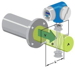
Magnetic flow meters work based on Faraday’s Law of Electromagnetic Induction. According to this principle, when a conductive medium passes through a magnetic field B, a voltage E is generated which is proportional to the velocity v of the medium, the density of the magnetic field, and the length of the conductor.
In a magnetic flow meter, a current is applied to wire coils mounted within or outside the meter body to generate a magnetic field. The liquid flowing through the pipe acts as the conductor and this induces a voltage that is proportional to the average flow velocity.
This voltage is detected by sensing electrodes mounted in the Magflow meter body and sent to a transmitter which calculates the volumetric flow rate based on the pipe dimensions.
Mathematically, we can state Faraday’s law as
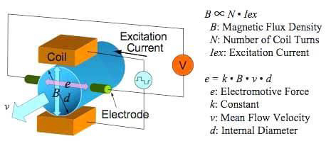
E is proportional to V x B x L
[E is the voltage generated in a conductor, V is the velocity of the conductor, B is the magnetic field strength and L is the length of the conductor].
It is very important that the liquid flow that is to be measured using the magnetic flow meter must be electrically conductive.
Faraday’s Law indicates that the signal voltage (E) is dependent on the average liquid velocity (V), the length of the conductor (D), and the magnetic field strength (B). The magnetic field will thus be established in the cross-section of the tube.
Basically, when the conductive liquid flows through the magnetic field, voltage is induced. To measure this generated voltage (which is proportional to the velocity of the flowing liquid), two stainless steel electrodes are used which are mounted opposite each other.
The two electrodes which are placed inside the flow meter are then connected to an advanced electronic circuit that has the ability to process the signal. The processed signal is fed into the microprocessor that calculates the volumetric flow of the liquid.
Electromagnetic Flow Meter Formula
Electromagnetic flow meters use Faraday’s law of electromagnetic induction to make a flow measurement.
Faraday’s law states that whenever a conductor of length ‘l’ moves with a velocity ‘v’ perpendicular to a magnetic field ‘B’, an emf ‘e’ is induced in a mutually perpendicular direction which is given by
e = Blv …(eq1)
where B = Magnetic flux density (Wb/m2) l = length of conductor (m) v = Velocity of the conductor (m/s)
The volume flow rate Q is given by
Q = (πd2/4) v …(eq2)
where d = diameter of the pipe v = average velocity of flow (conductor velocity in this case)
From equation (eq1)
v = e/Bl
Q = πd2e/4Bl
Q = Ke
where K is a meter constant.
Thus the volume flow rate is proportional to the induced emf. In Practical applications, we have to enter the meter constant ‘K’ value in the magnetic flow meter which is available in the vendor catalog/manual.
Industrial Applications
Electromagnetic flow meters are widely used for measuring conductive liquids across various industries due to their high accuracy, no moving parts, and low maintenance.
Water & Wastewater Industry
• Raw water intake measurement
• Treated water distribution
• Sewage and sludge flow monitoring
• Effluent discharge measurement
• Treated water distribution
• Sewage and sludge flow monitoring
• Effluent discharge measurement
Chemical Industry
• Corrosive liquid flow measurement (acids, alkalis)
• Chemical dosing and batching systems
• Process control in reactors and pipelines
• Chemical dosing and batching systems
• Process control in reactors and pipelines
Food & Beverage Industry
• Milk, juice, beer, and soft drink flow measurement
• Hygienic applications (CIP/SIP systems)
• Liquid ingredient dosing
• Hygienic applications (CIP/SIP systems)
• Liquid ingredient dosing
Pharmaceutical Industry
• Sterile liquid flow monitoring
• Precise dosing of liquid medicines
• Cleanroom process applications
• Precise dosing of liquid medicines
• Cleanroom process applications
Power Plants
• Cooling water flow measurement
• Boiler feed water monitoring
• Flue gas desulfurization (FGD) slurry flow
• Boiler feed water monitoring
• Flue gas desulfurization (FGD) slurry flow
Pulp & Paper Industry
• Pulp stock flow measurement
• Chemical liquor monitoring
• Coating and bleaching process control
• Chemical liquor monitoring
• Coating and bleaching process control
Mining & Metals Industry
• Slurry flow measurement (abrasive fluids)
• Mineral processing pipelines
• Tailings and waste flow monitoring
• Mineral processing pipelines
• Tailings and waste flow monitoring
Oil & Gas (Limited Use)
• Water injection systems
• Produced water measurement
• Not suitable for hydrocarbons due to non-conductivity
• Produced water measurement
• Not suitable for hydrocarbons due to non-conductivity
Irrigation & Agriculture
• Canal and pipeline water flow measurement
• Fertilizer dosing systems
• Groundwater monitoring
• Fertilizer dosing systems
• Groundwater monitoring
Textile Industry
• Dyeing and chemical dosing processes
• Water consumption monitoring
• Water consumption monitoring
Technical Specifications
| Parameter | Details |
|---|---|
| Nominal Diameter | 15 – 2000 mm |
| Velocity Range | 0.5 – 10 m/s |
| Accuracy | ±0.5%, ±1%R (< DN20), ±0.2% (> DN25) |
| Medium Conductivity |
Actual Conductivity ≥ 30 μS/cm (Standard) Conductivity > 5 μS/cm (Optional ≤ DN150) |
| Nominal Pressure | 1.0 ~ 4.0 MPa |
| Environment Temperature |
LCD Display: -10°C ~ +55°C OLED Display: -30°C ~ +55°C |
| Medium Temperature |
CR: 0 ~ 80°C PTFE: 0 ~ 120°C FEP: 0 ~ 120°C PFA: -10 ~ 180°C FVMQ: 70 ~ 250°C PU: -20 ~ 60°C |
| Output Signal | 4–20 mA; Pulse / Frequency 2KHz (Default), 5KHz (Max) |
| Cable Entry Size | M20×1.5 (Standard waterproof connector, optional explosion-proof metal connector) |
| Galvanic Isolation | Available |
| Surge Arrestor | Optional accessory |
| Supply Voltage |
4-wire Type 110 / 220 VAC (100–240 VAC), 50/60 Hz 24 VDC ±10% Power Dissipation ≤ 15 VA |
| Digital Communication | RS-485, Modbus-RTU Protocol |
| Electrode Materials | SS316L, Hastelloy B, Titanium, Tantalum, Platinum |
| Electrode Type | Interpolation / Extrapolating (customized) |
| Number of Electrodes | 3–4 electrodes (2 measuring + 1 grounding electrode) |
| Flange Standard | DIN, ANSI or others |
| Connecting Flange Material | Carbon Steel (Standard), SS304 / SS316 optional |
| Grounding Ring Material | Stainless Steel (Standard), Hastelloy C, Tantalum, Titanium optional |
| Transmitter Material | Die-cast Aluminum (Standard) / SS304 (Optional) |
| Housing Material |
Flow Tube: SS304 Flange / Sensor Housing: Carbon Steel, SS304 / SS316 optional |
| Protection Class |
Separate Body Type: IP67 / IP68 (Epoxy sealed) Integrated Type: IP65 |
| Cable Length | 10 m standard connecting cable (Optional: 1 – 50 m) |
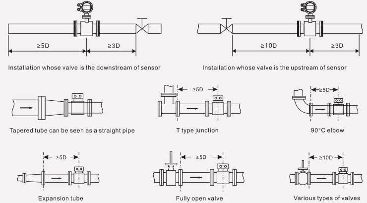
Installation
Straight pipe length requirements
Recommended mounting position
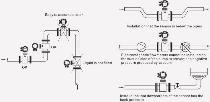
The connection which is easy to clean pipe

Flow Range Table
| DN (mm) | Flow Rate (m³/h) | ||||||||||
|---|---|---|---|---|---|---|---|---|---|---|---|
| 0.5 | 1 | 2 | 3 | 4 | 5 | 6 | 7 | 8 | 9 | 10 | |
| 15 | 0.3 | 0.6 | 1.3 | 1.9 | 2.5 | 3.2 | 3.8 | 4.5 | 5.1 | 5.7 | 6.4 |
| 20 | 0.6 | 1.1 | 2.3 | 3.4 | 4.5 | 5.7 | 6.8 | 7.9 | 9 | 10.2 | 11.3 |
| 25 | 0.9 | 1.8 | 3.5 | 5.3 | 7.1 | 8.8 | 10.6 | 12.4 | 14.1 | 15.9 | 17.7 |
| 32 | 1.4 | 2.9 | 5.8 | 8.7 | 11.6 | 14.5 | 17.4 | 20.3 | 23.2 | 26.1 | 29 |
| 40 | 2.3 | 4.5 | 9 | 13.6 | 18.1 | 22.6 | 27.1 | 31.7 | 36.2 | 40.7 | 45.2 |
| 50 | 3.5 | 7.1 | 14.1 | 21.2 | 28.3 | 35.3 | 42.4 | 49.5 | 56.5 | 63.6 | 70.7 |
| 65 | 6 | 11.9 | 23.9 | 35.8 | 47.8 | 59.7 | 71.7 | 83.6 | 95.6 | 107.5 | 119.5 |
| 80 | 9 | 18.1 | 36.2 | 54.3 | 72.4 | 90.5 | 108.6 | 126.7 | 144.8 | 162.9 | 181 |
| 100 | 14.1 | 28.3 | 56.5 | 84.8 | 113.1 | 141.4 | 169.6 | 197.9 | 226.2 | 254.5 | 282.7 |
| 125 | 22.1 | 44.2 | 88.4 | 132.5 | 176.1 | 220.9 | 265.1 | 309.2 | 353.4 | 397.6 | 441.8 |
| 150 | 31.8 | 63.6 | 127.2 | 190.8 | 254.5 | 318.1 | 381.7 | 445.3 | 508.9 | 572.5 | 636.2 |
| 200 | 56.5 | 113.1 | 226.2 | 339.3 | 452.4 | 565.5 | 678.6 | 791.7 | 904.8 | 1017.9 | 1131 |
Model Selection Table